Parrondo's Paradox¶

A fun hands-on example to understand Markov Models.

Introduction¶

Parrondo's paradox is a mind-blowing mental experiment in which the combination of two different losing games can become in a wining one. $$ L_{ose} + L_{ose} = W_{in}?$$

There's a lot of interesting literature around it. You can search for it in the internet, but I'll just explain the most simple example in terms of two games played with biased coins.

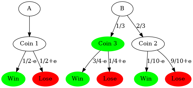
In Game A, we toss a biased coin, Coin 1, with probability of winning $ P_{1}=(1/2)-\epsilon$.

If $\epsilon >0$, this is clearly a losing game in the long run.
In Game B, we first determine if our capital is a multiple of some integer $M$.

2.1. If it is, we toss a biased coin, Coin 2, with probability of winning $P_{2}=(1/10)-\epsilon$.

2.2. If it is not, we toss another biased coin, Coin 3, with probability of winning $P_{3}=(3/4)-\epsilon$.

At each turn, we'll be able to choose playing game A or B.

Let's try to draw it and understand the very basic probabilities involved.

In [1]:

import graphviz
d=graphviz.Digraph()
for idx, i in enumerate(('Win', 'Lose', 'Win', 'Lose', 'Win', 'Lose')):
    d.node(str(idx),i, color=['green', 'red'][idx % 2], style='filled')

d.edge('A', 'Coin 1')
d.edge('Coin 1', '0', '1/2-e')
d.edge('Coin 1', '1', '1/2+e')
d.edge('B', 'Coin 2', 'C%M != 0')
d.edge('B', 'Coin 3', 'C%M == 0')
d.edge('Coin 2', '2', '1/10-e')
d.edge('Coin 2', '3', '9/10+e')
d.edge('Coin 3', '4', '3/4-e')
d.edge('Coin 3', '5', '1/4+e')

In [2]:

from IPython.display import Image

Image(d.render(filename='parr1.png', format='png'))

Out[2]:

In [3]:

import graphviz
d=graphviz.Digraph()
for idx, i in enumerate(('Win', 'Lose', 'Win', 'Lose', 'Win', 'Lose')):
    d.node(str(idx),i, color=['green', 'red'][idx % 2], style='filled')
d.node('Coin 3','Coin 3', color='green', style='filled')
d.edge('A', 'Coin 1')
d.edge('Coin 1', '0', '1/2-e')
d.edge('Coin 1', '1', '1/2+e')
d.edge('B', 'Coin 2', '2/3')
d.edge('B', 'Coin 3', '1/3')
d.edge('Coin 2', '2', '1/10-e')
d.edge('Coin 2', '3', '9/10+e')
d.edge('Coin 3', '4', '3/4-e')
d.edge('Coin 3', '5', '1/4+e')

In [4]:

Image(d.render(filename='parr2.png', format='png'))

Out[4]:

A Little bit of statistics show that B is also a losing game:

$$P(W) = P(W|C_3) \cdot P(C_3) + P(W|C_2) \cdot P(C_2)$$$$P(L) = P(L|C_3) \cdot P(C_3) + P(L|C_2) \cdot P(C_2)$$

In [5]:

epsilon = 0.005
P_W = (3/4 - epsilon)*1/3 + (1/10 - epsilon) * 2/3
P_W

Out[5]:

0.31166666666666665

In [6]:

P_L = (1/4 + epsilon)*1/3 + (9/10 + epsilon) * 2/3
P_L

Out[6]:

0.6883333333333334

Now with Python¶

Let's just code the coin's behaviour:

In [7]:

import random

def coin_1(epsilon):
    if random.random() < 0.5 - epsilon:
        return 1
    else:
        return -1
def coin_2(epsilon):
    if random.random() < 0.1 - epsilon:
        return 1
    else:
        return -1
def coin_3(epsilon):
    if random.random() < 0.75 - epsilon:
        return 1
    else:
        return -1

And now the whole game:

In [8]:

class Parrondo(object):
    
    def game_A(self):
        self.coins.append(1)
        return coin_1(self.epsilon)
        
    def game_B(self):
        if self.capital % self.modulus == 0:
            self.coins.append(2)
            return coin_2(self.epsilon)           
        else:
            self.coins.append(3)
            return coin_3(self.epsilon)   
    
    def __init__(self, epsilon = 0.005, modulus = 3):
        random.seed(0)
        self.epsilon = epsilon
        self.capital_history = []
        self.capital = 0
        self.modulus = modulus
        self.coins = []
    @property
    def capital(self):
        return self.capital_history[-1]
    @capital.setter
    def capital(self, value):
        self.capital_history.append(value)        
    
    def play(self, coins):
        for c in coins:
            if c == 'R':
                c = 'AB'[random.randint(0,1)]
            if c == 'A':
                result = self.game_A()
                self.capital += result
            elif c == 'B':
                result = self.game_B()
                self.capital += result
        return '%s%s' % (
            c,
            {-1: 'l', 1: 'w'}[result]
        )

In [9]:

tries = 10000

Let's try playing each game separately

In [10]:

p1=Parrondo()
p1.play('AAAA'*tries)
p1.capital

Out[10]:

-512

In [11]:

p2=Parrondo()
p2.play('BBBB'*tries)
p2.capital

Out[11]:

-322

What about periodically mixing games?¶

In [12]:

p3=Parrondo()
p3.play('ABAB'*tries)
p3.capital

Out[12]:

-286

In [13]:

p4=Parrondo()
p4.play('ABAA'*tries)
p4.capital

Out[13]:

And a random strategy

In [14]:

pR=Parrondo()
pR.play('RRRR'*tries)
pR.capital

Out[14]:

We can plot the behaviour of each strategy to have a more graphical understanding of what is happening:

In [15]:

import pandas

In [16]:

df = pandas.DataFrame()
df['A'] = p1.capital_history
df['B'] = p2.capital_history
df['ABAB'] = p3.capital_history
df['ABAA'] = p4.capital_history
df['Random'] = pR.capital_history

In [17]:

%matplotlib inline
import matplotlib.style
matplotlib.style.use('seaborn')

In [18]:

df.plot(figsize=(15,5))

Out[18]:

An intelligent player¶

Let's say I know my capital and the rules of the game. The evident strategy is playing game A if my capital is multiple of 3 and game B in other case:

In [19]:

pI = Parrondo()
for i in df['A'][:-1]:
    if pI.capital % 3 == 0:
        pI.play('A')
    else:
        pI.play('B')

In [20]:

df['Intelligent'] = pI.capital_history

In [21]:

df.plot(figsize=(15,5))

Out[21]:

The Pelayo's Model¶

But what we are doing with that "intelligent" player is a little bit like cheating. Let's try with a more realistic scenario.

Let's say I don't know the internal rules of the game, but I will just play and try to learn how the system behaves. My hope is to find some kind of statistical bias in the game and use it for my own benefit.

I've called it the Pelayo's strategy in honour of a family which gained fame in the 90s for exploiting roulette games in casinos. Again, there's a lot of interesting information in the internet about their story.

In [22]:

d=graphviz.Digraph()
for idx, i in enumerate(('Win', 'Lose', 'Win', 'Lose', 'Win', 'Lose')):
    d.node(str(idx),i, color=['green', 'red'][idx % 2], style='filled')
d.node('Coin 3','???')
d.node('Coin 2','???')
d.node('Coin 1','???')
d.edge('A', 'Coin 1')
d.edge('Coin 1', '0', '???')
d.edge('Coin 1', '1', '???')
d.edge('B', 'Coin 2', '???')
d.edge('B', 'Coin 3', '???')
d.edge('Coin 2', '2', '???')
d.edge('Coin 2', '3', '???')
d.edge('Coin 3', '4', '???')
d.edge('Coin 3', '5', '???')
Image(d.render(filename='parr1.png', format='png'))

Out[22]:

Let's build a Markov model¶

In probability theory, a Markov model is a stochastic model for randomly changing systems. The main assumption in a Markov chain is that future states depend only on the current state, not on the events that occurred before it. One of the most common examples is trying to predict if tomorrow will be rainy or sunny knowing only if today is rainy or sunny.

At this point, I'll introduce the following notation. My possible states will be $A_w$, $A_l$, $B_w$ and $B_l$, which mean winning or losing when playing game $A$ or $B$.

Let's define a small class to store a simple probabilistic model

In [23]:

class Model(object):
    __probs = None
    def __init__(self):
        self.model = pandas.DataFrame()
        states = ('Aw', 'Al', 'Bw', 'Bl')
        for i in states:
            self.model[i]=[0,0,0,0]
        self.model.index=states
    @property
    def probs(self):
        '''This property will return a dictionary with the 
        probabilities for wining in next movement in terms of last one'''
        if self.__probs is not None:
            return self.__probs
        self.__probs = pandas.DataFrame()
        for i in self.model.columns:
            self.__probs[i] = [
                self.model[i]['Aw']/(self.model[i]['Aw']+self.model[i]['Al']),
                self.model[i]['Bw']/(self.model[i]['Bw']+self.model[i]['Bl'])
            ]
        self.__probs.index = ['A','B']
        return self.__probs
    
    def update(self, last, now):
        '''Update function feeds the model with new training results'''
        self.__probs = None
        self.model[last][now]+=1
    
    def bet(self, last):
        '''Returns the game with higher winning probabilities given last state'''
        return self.probs[last].idxmax()

The only information we're currently storing in our model is the amount of transitions from one state to the next one. We can represent it in a transition matrix which is initialized to zeros.

In [24]:

model=Model()
model.model

Out[24]:

	Aw	Al	Bw	Bl
Aw	0	0	0	0
Al	0	0	0	0
Bw	0	0	0	0
Bl	0	0	0	0

Training the model with random plays¶

For training the model we'll just play randomly (or look how others play) and store the results.

In [25]:

p_train=Parrondo()
last = p_train.play('R')
for i in range(100000):
    now = p_train.play('R')
    model.update(last,now)
    last=now

In [26]:

model.model

Out[26]:

	Aw	Al	Bw	Bl
Aw	6101	6194	6345	5811
Al	6182	6523	6658	6081
Bw	5943	7294	4980	7905
Bl	6224	5433	8139	4187

This trained transition matrix means only how many times we have reached a certain state given a previous one.

For example, we have reached stated $A_w$ coming from state $A_l$:

In [27]:

model.model['Al']['Aw']

Out[27]:

By just normalizing, we can easily guess transition probabilities:

In [28]:

dm = graphviz.Digraph()
states = model.model.columns
for state in states:
    if 'l' in state:
        dm.node(state, state, color='red', style='filled')
    else:
        dm.node(state, state, color='green', style='filled')
for last in states:
    weights = model.model[last]/model.model[last].sum()    
    for bet in states:
        dm.edge(last, bet, '%.3f' % weights[bet])
Image(dm.render(filename='parr1.png', format='png'))

Out[28]:

The most valuable results we can find in here are the probabilities of winning if we choose $A$ or $B$ games coming from a known state $A_l$, $A_w$, $B_l$, $B_w$: $$\left(\begin{array}[cccc] PP(W|A|A_w) & P(W|A|A_l) & P(W|A|B_w) & P(W|A|B_l)\cr P(W|B|A_w) & P(W|B|A_l) & P(W|B|B_w) & P(W|B|B_l) \end{array}\right)$$

In [29]:

model.probs

Out[29]:

	Aw	Al	Bw	Bl
A	0.496703	0.487065	0.487964	0.488648
B	0.488452	0.573112	0.379602	0.653738

With this, we can now design a simple strategy by choosing the game with highest wining probability taking only into account previous state.

In [30]:

p_winner = Parrondo()
last = p_winner.play('R')
for i in df['A'][:-2]:
    last = p_winner.play(model.bet(last))

In [31]:

df['MModel_O1'] = p_winner.capital_history
df.plot(figsize=(15,5))

Out[31]:

As you can see, this model is obviously not as efficient as the "intelligent" one, but reveals as much better than any other "legal" model.

In [32]:

i=df.pop('Intelligent')

Higher order models¶

The initial assumption of Markov Models can be relaxed (and so the model enriched) with higher order Markov Chains (taking into account more than one previous state) or with Hidden Markov Models (taking into account non-observable states).

Let's try with higher order Markov Models, considering not one but several previous steps in the chain. For this purpose, we'll need an $N$-dimensional array for order-$N$ models, so we'll modify our class to use a nested dict to store the statistics instead of a bidimensional matrix.

In [33]:

from functools import reduce
import operator

class Model2(object):
    __probs = None
    def __init__(self):
        self.model = {}
        self.states = ('Aw', 'Al', 'Bw', 'Bl')
    
    def __add_value(self, state_list, value = 1):
        """Increase a probability value in a nested dict."""
        root = self.model
        for state in state_list:
             root = root.setdefault(state, {'__value__': 0})
        root['__value__'] = value + self.__get_value(state_list) 
        
    def __get_value(self, state_list):
        """Access a probability value in a nested dict."""
        root = self.model
        return reduce(operator.getitem, state_list, root).get('__value__', 0)
    
    def probs(self, state_list):
        '''Returns the probability of winning in next turn for both A and B games'''
        out={}
        for last in self.states:
            out[last] = self.__get_value(state_list + [last])
        return {
                'A': out['Aw']/(out['Aw']+out['Al']),
                'B': out['Bw']/(out['Bw']+out['Bl'])
                }
    
    def update(self, state_list):
        self.__add_value(state_list)
    
    def bet(self, state_list):
        '''Choose next movement based on stored stats'''
        p = self.probs(state_list)
        return max(p.items(), key=lambda x: x[1])[0]

Now we'll train the new model in the same manner as previous one but injecting 2, 3, 4, 5 and 6 consequent previous states instead of only one:

In [34]:

max_range=8
model2=Model2()
p_train=Parrondo()
statelist=[]
for i in range(max_range):
    statelist.append(p_train.play('R'))
for i in range(1000000):
    statelist.append(p_train.play('R'))
    for i in range(max_range):
        model2.update(statelist[i:])
    p=statelist.pop(0)

Let's now play with all of them with the same game rules and see how they behave:

In [35]:

for i in range(5):
    max_range=i+2
    player1 =Parrondo()
    statelist=[]
    for i in range(max_range):
        statelist.append(player1.play('R'))
    for i in range(100000):
        b=model2.bet(statelist)
        statelist.append(player1.play(b))
        statelist.pop(0)
    df['MModel_O%s' % max_range] = player1.capital_history[:len(df['A'])]

In [36]:

df.plot(figsize=(15,5))

Out[36]:

Obviously, models of higher orders lead to better results but also increase model's complexity, amount of training required and so computational cost.

Even if this use case is a toy model just for fun and the models look quite simple, this techniques have demonstrated to be really usefull in interesting and profitable fields such as protocol monitoring, anomaly detection, automated root cause analysis or natural language processing.

Hope you enjoyed.

Some random references around this topics:

The Awesome Adventures of a Drinking Bird